Measure pairwise coupling¶

Question¶

How far does one trace lead another, and is the lag stable?

See every package-generated example · Read the complete analysis pipeline

When to use¶

Use this for exactly two rhythmic traces on one shared time grid when stable phase lag and phase locking are the targets.

Example figure¶

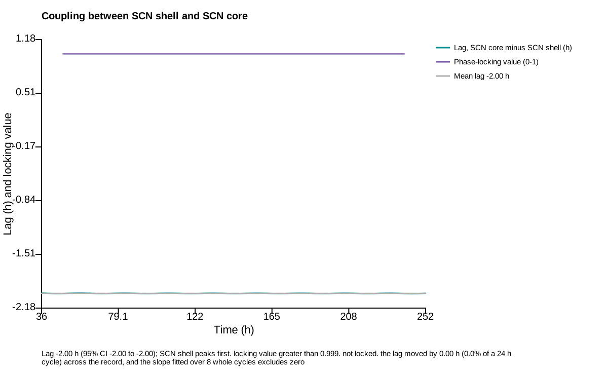
Measure pairwise coupling output generated by Circadian Workbench

This deterministic example is calculated by the coupling action and drawn by render_coupling_svg, the same renderer used for publication export. Empty or withheld elements are therefore visible exactly as they are in a real result.

import circadian_workbench as cw

cw.trace(hours, shell, name="SCN shell").coupling(core)

Required inputs and controls¶

The public function is the registered action below. settings= is accepted as a friendlier alias for config= by cw.call; the calculation stores the complete normalized config in provenance.

Function reference¶

cw.call("coupling", series_a, series_b, hours, config=None)

Arguments and parameters¶

Name	Type	Required	Default	Units	Meaning
`series_a`	object	yes	—	recording units	The first trace: {'label': 'left lobe', 'values': [...]} on the shared hours grid. A [label, values] array works too. The label is reported back as the one that leads or lags, so make it the name you would use in a figure.
`series_b`	object	yes	—	recording units	The second trace, same shape as series_a and on the same hours grid. The reported lag is negative when series_a peaks first.
`hours`	array	yes	—	hours	The shared time grid the traces are sampled on, in hours from the start of the recording.
`config`	object	no	`null`	-	Partial analysis config. Missing keys fall back to analysis.DEFAULT_CONFIG and out-of-range values are clamped silently — run describe_config for every key, its default and its allowed values, or normalize_config to see what a given config actually becomes.

Every nested config key, default, allowed value, and purpose is listed in the complete configuration reference.

How it works¶

Band-limited Hilbert phases are subtracted pointwise. The circular mean gives lag, the resultant length gives phase-locking value, and sliding windows plus leave-one-cycle-out intervals test stability.

$$ \Delta\theta(t)=\theta_B(t)-\theta_A(t),\qquad PLV=\left|\frac{1}{N}\sum_t e^{i\Delta\theta(t)}\right| $$

Implementation: coupling.py::coupling.

Outputs and interpretation¶

The result reports lag and interval, leading trace, phase-locking value, drift and interval, windowed trajectories, overlap, cycles, locking verdict, and notes.

cw.call returns a Result: use .data for calculated values, .warnings for scientific qualifications, .provenance for version and input identity, .script for an equivalent replay script, and .files for saved outputs.

Limitations¶

Phase locking is association, not causal coupling. No p value is assigned to phase-locking value, and cross-correlation lag is deliberately not used because waveform and trend can mimic it.

Example¶

The figure above is a real package result from a seeded, redistributable synthetic dataset. Its audited project bundle retains figure_data.csv, a standalone plot.py, source hashes, an editable SVG, and a rendered preview.

Methods text¶

The two aligned traces were compared by their band-limited Hilbert phase difference; circular lag, phase-locking value, drift, sliding-window stability, and leave-one-cycle-out uncertainty were reported.