Fit a phase response curve¶

Question¶

How does stimulus timing change the clock?

See every package-generated example · Read the complete analysis pipeline

When to use¶

Use this when independent animals received a timed stimulus and the response must be related to each animal's circadian phase.

Example figure¶

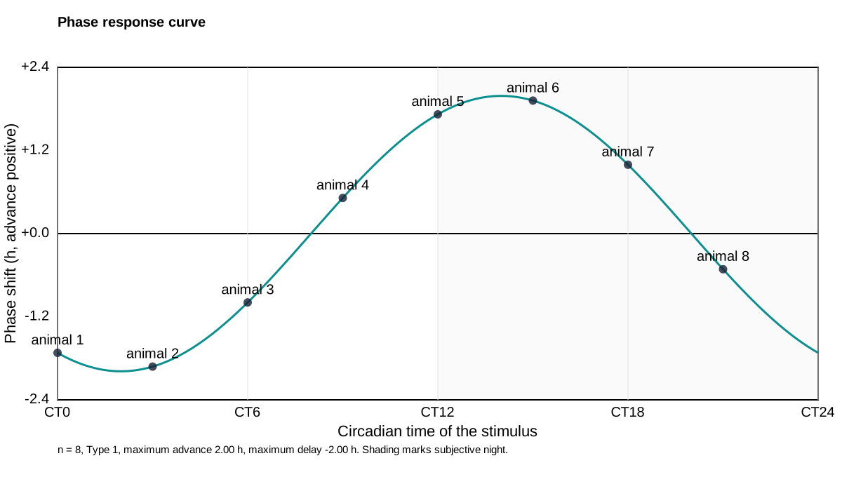
Fit a phase response curve output generated by Circadian Workbench

This deterministic example is calculated by the phase_response_curve action and drawn by render_phase_response_svg, the same renderer used for publication export. Empty or withheld elements are therefore visible exactly as they are in a real result.

import circadian_workbench as cw

cw.call("phase_response_curve", animals=animals)

Required inputs and controls¶

The public function is the registered action below. settings= is accepted as a friendlier alias for config= by cw.call; the calculation stores the complete normalized config in provenance.

Function reference¶

cw.call("phase_response_curve", animals, config=None)

Arguments and parameters¶

Name	Type	Required	Default	Units	Meaning
`animals`	array of objects	yes	—	-	One entry per animal in the pulse experiment. Either a record to score -- {'recording': spec, 'stimulus': '2026-01-08 18:00', 'label': 'm01', 'config': {...}} -- or a point already scored elsewhere: {'circadian_time': 15.2, 'shift_hours': -1.4, 'label': 'm01'}. A record needs fit1_start/fit1_end before the pulse and fit2_start/fit2_end after it in its config, and 'stimulus' is the wall-clock time the pulse landed (or hours from the start of the record's first day). An animal whose pre-stimulus fit is too short is dropped with a warning rather than failing the cohort.
`config`	object	no	`null`	-	Partial analysis config. Missing keys fall back to analysis.DEFAULT_CONFIG and out-of-range values are clamped silently — run describe_config for every key, its default and its allowed values, or normalize_config to see what a given config actually becomes.

Every nested config key, default, allowed value, and purpose is listed in the complete configuration reference.

How it works¶

Pre-stimulus onset regression supplies circadian time and the before/after marker fits supply phase shift. A periodic harmonic regression is then fitted across animals using the advance-positive Aschoff convention.

$$ \Delta(\phi)=a_0+\sum_{h=1}^{H}\left[a_h\cos!\left(\frac{2\pi h\phi}{24}\right)+b_h\sin!\left(\frac{2\pi h\phi}{24}\right)\right] $$

Implementation: phase_response.py::phase_response_curve.

Outputs and interpretation¶

The curve includes animal points, fitted values, coefficients, uncertainty, advance and delay extrema, dead-zone estimate, phase coverage, and type-classification diagnostics.

cw.call returns a Result: use .data for calculated values, .warnings for scientific qualifications, .provenance for version and input identity, .script for an equivalent replay script, and .files for saved outputs.

Limitations¶

Animals without adequate pre/post fits are dropped and named. A curve needs the configured minimum animals and phase coverage; clock-time stimulus bins are not a substitute for circadian time.

Example¶

The figure above is a real package result from a seeded, redistributable synthetic dataset. Its audited project bundle retains figure_data.csv, a standalone plot.py, source hashes, an editable SVG, and a rendered preview.

Methods text¶

Per-animal circadian stimulus time and phase shift were scored from declared marker fits and modelled by periodic harmonic regression using the advance-positive Aschoff convention.