Map phase across space¶

Question¶

Is phase graded across the tissue?

See every package-generated example · Read the complete analysis pipeline

When to use¶

Use this after phase has been measured for spatially located cells or regions and a tissue-scale gradient is the target.

Example figure¶

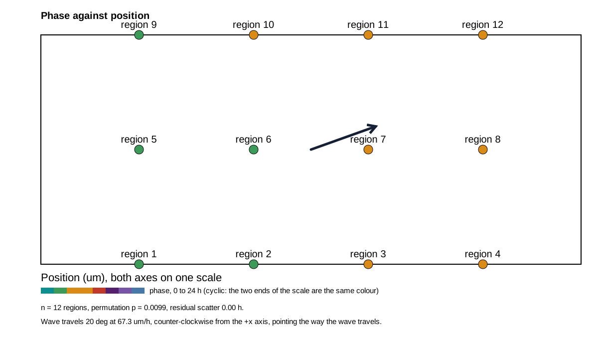
Map phase across space output generated by Circadian Workbench

This deterministic example is calculated by the phase_map action and drawn by render_phase_map_svg, the same renderer used for publication export. Empty or withheld elements are therefore visible exactly as they are in a real result.

import circadian_workbench as cw

cw.call("phase_map", points=regions, position_units="um")

Required inputs and controls¶

The public function is the registered action below. settings= is accepted as a friendlier alias for config= by cw.call; the calculation stores the complete normalized config in provenance.

Function reference¶

cw.call("phase_map", points, config=None, period_hours=None, position_units='um')

Arguments and parameters¶

Name	Type	Required	Default	Units	Meaning
`points`	array	yes	—	hours and position units	One entry per region, each carrying a phase and a position: [{'label': 'left', 'phase_hours': 6.2, 'x': 120, 'y': 340}, ...]. A list of [label, phase_hours, x, y] arrays works too. The phases are ones the caller already measured -- acrophases from a cosinor, peak times, onsets -- and the positions are region centroids in whatever unit position_units names. Six regions is the floor; below it the plane is fitted but never tested.
`config`	object	no	`null`	-	Partial analysis config. Missing keys fall back to analysis.DEFAULT_CONFIG and out-of-range values are clamped silently — run describe_config for every key, its default and its allowed values, or normalize_config to see what a given config actually becomes.
`period_hours`	float	no	`null`	hours	The cycle the phases live on. Omit to use the config's period_hours (24 h by default). A free-running cohort should pass its own tau, so that 'one cycle' means one of the animals' cycles rather than one solar day. `splitting` uses it for a second purpose that is the same idea: the period the resolution element P**2/T is worked out at, which sets how far apart two components must be before that record can show them to differ.
`position_units`	string	no	`"um"`	-	What the x and y in points are measured in: 'um', 'px', 'mm'. It travels through to the reported speed, which comes back in these units per hour. Nothing is converted -- this is a label, so pass the unit the positions are actually in.

Every nested config key, default, allowed value, and purpose is listed in the complete configuration reference.

How it works¶

Circular phase is regressed jointly on x and y position. Permuting phase labels supplies significance while a collinearity guard rejects effectively one-dimensional layouts.

$$ \theta_i=\theta_0+b x_i+c y_i+\epsilon_i,\qquad g=\sqrt{b^2+c^2} $$

Implementation: spatial.py::phase_map.

Outputs and interpretation¶

The result reports point phases, fitted phases, gradient vector and direction, wavelength, propagation speed, goodness of fit, permutation p value, geometry diagnostics, and units.

cw.call returns a Result: use .data for calculated values, .warnings for scientific qualifications, .provenance for version and input identity, .script for an equivalent replay script, and .files for saved outputs.

Limitations¶

Fewer than the configured six points are refused. Near-collinear coordinates cannot identify a two-dimensional gradient, and the position unit is labelled rather than converted.

Example¶

The figure above is a real package result from a seeded, redistributable synthetic dataset. Its audited project bundle retains figure_data.csv, a standalone plot.py, source hashes, an editable SVG, and a rendered preview.

Methods text¶

Circular phase was modelled as a planar function of x and y position; phase-label permutation tested the spatial gradient and near-collinear layouts were rejected.