Track phase and period¶

Question¶

Does phase or period drift through the recording?

See every package-generated example · Read the complete analysis pipeline

When to use¶

Use this when a single average period would hide drift, transients, or time-local changes in phase.

Example figure¶

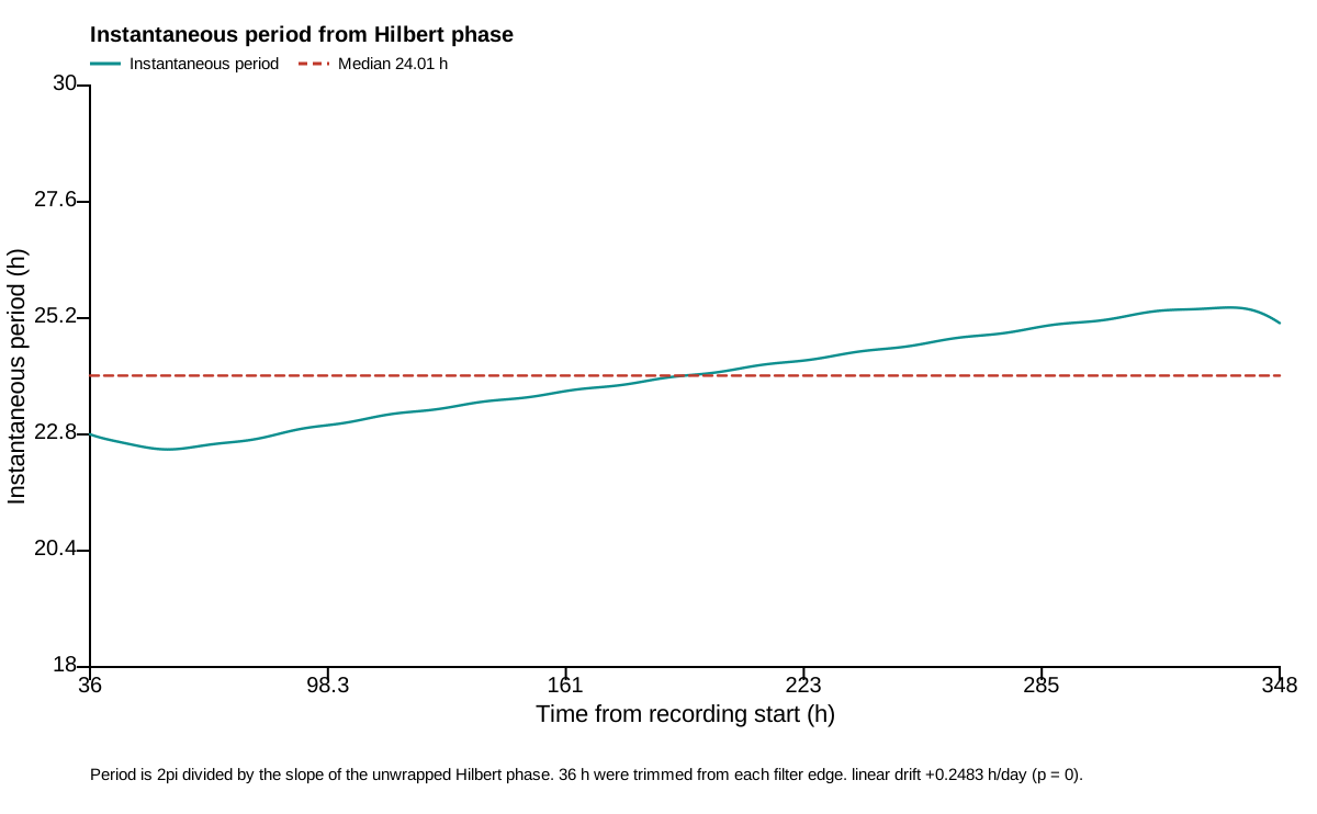
Track phase and period output generated by Circadian Workbench

This deterministic example is calculated by the instantaneous_phase action and drawn by render_instantaneous_phase_svg, the same renderer used for publication export. Empty or withheld elements are therefore visible exactly as they are in a real result.

import circadian_workbench as cw

cw.call("instantaneous_phase", recording={"path": "mouse01.awd"})

Required inputs and controls¶

The public function is the registered action below. settings= is accepted as a friendlier alias for config= by cw.call; the calculation stores the complete normalized config in provenance.

Function reference¶

cw.call("instantaneous_phase", recording, config=None)

Arguments and parameters¶

Name	Type	Required	Default	Units	Meaning
`recording`	recording spec	yes	—	-	The record to analyse: {'path': 'data/m01.awd'} (a bare path string also works), {'demo': true} for the built-in deterministic record, {'inline': {'filename': ..., 'text': ...}} for tabular text, {'trace': {'hours': [...], 'values': [...], 'name': ...}} for one elapsed-time trace, or {'channels': {'hours': [...], 'values': {'reporter_a': [...], 'reporter_b': [...]}}} for several measurements from one subject.
`config`	object	no	`null`	-	Partial analysis config. Missing keys fall back to analysis.DEFAULT_CONFIG and out-of-range values are clamped silently — run describe_config for every key, its default and its allowed values, or normalize_config to see what a given config actually becomes.

Every nested config key, default, allowed value, and purpose is listed in the complete configuration reference.

How it works¶

A band-limited analytic signal is formed with the Hilbert transform. Its angle is unwrapped into phase, its magnitude gives analytic amplitude, and the local phase slope gives instantaneous period after unreliable filter edges are trimmed.

$$ z(t)=x(t)+i\mathcal H[x(t)],\qquad P_{\mathrm{inst}}(t)=\frac{2\pi}{d\theta/dt} $$

Implementation: instantaneous.py::instantaneous_phase.

Outputs and interpretation¶

Time-aligned arrays contain phase, analytic amplitude, and instantaneous period; the summary reports the median period, drift slope, filter band, trimmed edge duration, and diagnostics.

cw.call returns a Result: use .data for calculated values, .warnings for scientific qualifications, .provenance for version and input identity, .script for an equivalent replay script, and .files for saved outputs.

Limitations¶

Phase and its derivative are unstable at low amplitude and near filter edges. The method needs a sufficiently sampled continuous trace and does not replace a global rhythmicity test.

Example¶

The figure above is a real package result from a seeded, redistributable synthetic dataset. Its audited project bundle retains figure_data.csv, a standalone plot.py, source hashes, an editable SVG, and a rendered preview.

Methods text¶

Instantaneous phase and amplitude were obtained from the band-limited analytic signal; phase was unwrapped, differentiated to obtain instantaneous period, and trimmed by the declared number of edge cycles.